01 [로지스틱 회귀 분석] 특징 데이터로 유방암 진단하기
사이킷런 의 유방암 진단 데이터셋 사용하기
import numpy as np
import pandas as pd

from sklearn.datasets import load_breast_cancer

b_cancer = load_breast_cancer()

print(b_cancer.DESCR)
.. _breast_cancer_dataset:

Breast cancer wisconsin (diagnostic) dataset
--------------------------------------------

**Data Set Characteristics:**

    :Number of Instances: 569

    :Number of Attributes: 30 numeric, predictive attributes and the class

    :Attribute Information:
        - radius (mean of distances from center to points on the perimeter)
        - texture (standard deviation of gray-scale values)
        - perimeter
        - area
        - smoothness (local variation in radius lengths)
        - compactness (perimeter^2 / area - 1.0)
        - concavity (severity of concave portions of the contour)
        - concave points (number of concave portions of the contour)
        - symmetry
        - fractal dimension ("coastline approximation" - 1)

        The mean, standard error, and "worst" or largest (mean of the three
        worst/largest values) of these features were computed for each image,
        resulting in 30 features.  For instance, field 0 is Mean Radius, field
        10 is Radius SE, field 20 is Worst Radius.

        - class:
                - WDBC-Malignant
                - WDBC-Benign

    :Summary Statistics:

    ===================================== ====== ======
                                           Min    Max
    ===================================== ====== ======
    radius (mean):                        6.981  28.11
    texture (mean):                       9.71   39.28
    perimeter (mean):                     43.79  188.5
    area (mean):                          143.5  2501.0
    smoothness (mean):                    0.053  0.163
    compactness (mean):                   0.019  0.345
    concavity (mean):                     0.0    0.427
    concave points (mean):                0.0    0.201
    symmetry (mean):                      0.106  0.304
    fractal dimension (mean):             0.05   0.097
    radius (standard error):              0.112  2.873
    texture (standard error):             0.36   4.885
    perimeter (standard error):           0.757  21.98
    area (standard error):                6.802  542.2
    smoothness (standard error):          0.002  0.031
    compactness (standard error):         0.002  0.135
    concavity (standard error):           0.0    0.396
    concave points (standard error):      0.0    0.053
    symmetry (standard error):            0.008  0.079
    fractal dimension (standard error):   0.001  0.03
    radius (worst):                       7.93   36.04
    texture (worst):                      12.02  49.54
    perimeter (worst):                    50.41  251.2
    area (worst):                         185.2  4254.0
    smoothness (worst):                   0.071  0.223
    compactness (worst):                  0.027  1.058
    concavity (worst):                    0.0    1.252
    concave points (worst):               0.0    0.291
    symmetry (worst):                     0.156  0.664
    fractal dimension (worst):            0.055  0.208
    ===================================== ====== ======

    :Missing Attribute Values: None

    :Class Distribution: 212 - Malignant, 357 - Benign

    :Creator:  Dr. William H. Wolberg, W. Nick Street, Olvi L. Mangasarian

    :Donor: Nick Street

    :Date: November, 1995

This is a copy of UCI ML Breast Cancer Wisconsin (Diagnostic) datasets.
https://goo.gl/U2Uwz2

Features are computed from a digitized image of a fine needle
aspirate (FNA) of a breast mass.  They describe
characteristics of the cell nuclei present in the image.

Separating plane described above was obtained using
Multisurface Method-Tree (MSM-T) [K. P. Bennett, "Decision Tree
Construction Via Linear Programming." Proceedings of the 4th
Midwest Artificial Intelligence and Cognitive Science Society,
pp. 97-101, 1992], a classification method which uses linear
programming to construct a decision tree.  Relevant features
were selected using an exhaustive search in the space of 1-4
features and 1-3 separating planes.

The actual linear program used to obtain the separating plane
in the 3-dimensional space is that described in:
[K. P. Bennett and O. L. Mangasarian: "Robust Linear
Programming Discrimination of Two Linearly Inseparable Sets",
Optimization Methods and Software 1, 1992, 23-34].

This database is also available through the UW CS ftp server:

ftp ftp.cs.wisc.edu
cd math-prog/cpo-dataset/machine-learn/WDBC/

.. topic:: References

   - W.N. Street, W.H. Wolberg and O.L. Mangasarian. Nuclear feature extraction
     for breast tumor diagnosis. IS&T/SPIE 1993 International Symposium on
     Electronic Imaging: Science and Technology, volume 1905, pages 861-870,
     San Jose, CA, 1993.
   - O.L. Mangasarian, W.N. Street and W.H. Wolberg. Breast cancer diagnosis and
     prognosis via linear programming. Operations Research, 43(4), pages 570-577,
     July-August 1995.
   - W.H. Wolberg, W.N. Street, and O.L. Mangasarian. Machine learning techniques
     to diagnose breast cancer from fine-needle aspirates. Cancer Letters 77 (1994)
     163-171.
b_cancer_df = pd.DataFrame(b_cancer.data, columns = b_cancer.feature_names)
b_cancer_df['diagnosis'] = b_cancer.target
b_cancer_df.head()
데이터셋의 크기와 독립 변수 X가 되는 피처에 대한 정보
print('유방암 진단 데이터셋 크기: ', b_cancer_df.shape)
유방암 진단 데이터셋 크기:  (569, 31)

b_cancer_df.info()
<class 'pandas.core.frame.DataFrame'>
RangeIndex: 569 entries, 0 to 568
Data columns (total 31 columns):
 #   Column                   Non-Null Count  Dtype
---  ------                   --------------  -----
 0   mean radius              569 non-null    float64
 1   mean texture             569 non-null    float64
 2   mean perimeter           569 non-null    float64
 3   mean area                569 non-null    float64
 4   mean smoothness          569 non-null    float64
 5   mean compactness         569 non-null    float64
 6   mean concavity           569 non-null    float64
 7   mean concave points      569 non-null    float64
 8   mean symmetry            569 non-null    float64
 9   mean fractal dimension   569 non-null    float64
 10  radius error             569 non-null    float64
 11  texture error            569 non-null    float64
 12  perimeter error          569 non-null    float64
 13  area error               569 non-null    float64
 14  smoothness error         569 non-null    float64
 15  compactness error        569 non-null    float64
 16  concavity error          569 non-null    float64
 17  concave points error     569 non-null    float64
 18  symmetry error           569 non-null    float64
 19  fractal dimension error  569 non-null    float64
 20  worst radius             569 non-null    float64
 21  worst texture            569 non-null    float64
 22  worst perimeter          569 non-null    float64
 23  worst area               569 non-null    float64
 24  worst smoothness         569 non-null    float64
 25  worst compactness        569 non-null    float64
 26  worst concavity          569 non-null    float64
 27  worst concave points     569 non-null    float64
 28  worst symmetry           569 non-null    float64
 29  worst fractal dimension  569 non-null    float64
 30  diagnosis                569 non-null    int64
dtypes: float64(30), int64(1)
memory usage: 137.9 KB
로지스틱 회귀 분석에 피처로 사용할 데이터를 평균이 0, 분산이 1이 되는 정규 분포 형태로 맞춘다.
from sklearn.preprocessing import StandardScaler
scaler = StandardScaler()

b_cancer_scaled = scaler.fit_transform(b_cancer.data)

print(b_cancer.data[0])
[1.799e+01 1.038e+01 1.228e+02 1.001e+03 1.184e-01 2.776e-01 3.001e-01
 1.471e-01 2.419e-01 7.871e-02 1.095e+00 9.053e-01 8.589e+00 1.534e+02
 6.399e-03 4.904e-02 5.373e-02 1.587e-02 3.003e-02 6.193e-03 2.538e+01
 1.733e+01 1.846e+02 2.019e+03 1.622e-01 6.656e-01 7.119e-01 2.654e-01
 4.601e-01 1.189e-01]

 print(b_cancer_scaled[0])
 [ 1.09706398 -2.07333501  1.26993369  0.9843749   1.56846633  3.28351467
  2.65287398  2.53247522  2.21751501  2.25574689  2.48973393 -0.56526506
  2.83303087  2.48757756 -0.21400165  1.31686157  0.72402616  0.66081994
  1.14875667  0.90708308  1.88668963 -1.35929347  2.30360062  2.00123749
  1.30768627  2.61666502  2.10952635  2.29607613  2.75062224  1.93701461]
분석 모델 구축 및 결과 분석
로지스틱 회귀를 이용하여 분석 모델 구축하기
from sklearn.linear_model import LogisticRegression
from sklearn.model_selection import train_test_split

#X, Y 설정하기
Y = b_cancer_df['diagnosis']
X = b_cancer_scaled

#훈련용 데이터와 평가용 데이터 분할하기
X_train, X_test, Y_train, Y_test = train_test_split(X, Y, test_size = 0.3, random_state = 0)

#로지스틱 회귀 분석: (1) 모델 생성
lr_b_cancer = LogisticRegression()

#로지스틱 회귀 분석: (2) 모델 훈련
lr_b_cancer.fit(X_train, Y_train)
LogisticRegression()

#로지스틱 회귀 분석: (3) 평가 데이터에 대한 예측 수행 -> 예측 결과 Y_predict 구하기
Y_predict = lr_b_cancer.predict(X_test)
생성한 모델의 성능 확인하기
from sklearn.metrics import confusion_matrix, accuracy_score
from sklearn.metrics import precision_score, recall_score, f1_score, roc_auc_score

#오차 행렬
confusion_matrix(Y_test, Y_predict)
array([[ 60,   3],
       [  1, 107]])

accuracy = accuracy_score(Y_test, Y_predict)
precision = precision_score(Y_test, Y_predict)
recall = recall_score(Y_test, Y_predict)
f1 = f1_score(Y_test, Y_predict)
roc_auc = roc_auc_score(Y_test, Y_predict)

print('정확도: {0:.3f}, 정밀도: {1:.3f}, 재현율: {2:.3f}, F1: {3:.3f}'.format(accuracy,precision,recall,f1))
정확도: 0.977, 정밀도: 0.973, 재현율: 0.991, F1: 0.982

print('ROC_AUC: {0:.3f}'.format(roc_auc))
ROC_AUC: 0.972
02 [결정 트리 분석 + 산점도/선형 회귀 그래프] 센서 데이터로 움직임 분류하기
데이터 탐색
훈련용과 테스트용 데이터셋 확인하기
import numpy as np
import pandas as pd

pd.__version__
1.3.5

#피처 이름 파일 읽어오기
feature_name_df = pd.read_csv('/features.txt', sep = '\s+', header = None, names = ['index', 'feature_name'], engine = 'python')

feature_name_df.head()
feature_name_df.shape
(561, 2)

#index 제거하고, feature_name만 리스트로 저장
feature_name = feature_name_df.iloc[:, 1].values.tolist()

feature_name[:5]
['tBodyAcc-mean()-X',
 'tBodyAcc-mean()-Y',
 'tBodyAcc-mean()-Z',
 'tBodyAcc-std()-X',
 'tBodyAcc-std()-Y']

 X_train = pd.read_csv('/X_train.txt', delim_whitespace=True, header=None, encoding='latin-1')
X_train.columns = feature_name
X_test = pd.read_csv('/X_test.txt', delim_whitespace=True, header=None, encoding='latin-1')
X_test.columns = feature_name
Y_train = pd.read_csv('/Y_train.txt', sep='\s+', header = None, names = ['action'], engine = 'python')
Y_test = pd.read_csv('/Y_test.txt', sep='\s+', header = None, names = ['action'], engine = 'python')

X_train.shape, Y_train.shape, X_test.shape, Y_test.shape
((7352, 561), (7352, 1), (2947, 561), (2947, 1))

X_train.head()
print(Y_train['action'].value_counts())
6    1407
5    1374
4    1286
1    1226
2    1073
3     986
Name: action, dtype: int64

label_name_df = pd.read_csv('/activity_labels.txt', sep = '\s+', header = None, names = ['index', 'label'], engine = 'python')

#index 제거하고, feature_name만 리스트로 저장
label_name = label_name_df.iloc[:, 1].values.tolist()

label_name
['WALKING',
 'WALKING_UPSTAIRS',
 'WALKING_DOWNSTAIRS',
 'SITTING',
 'STANDING',
 'LAYING']
분석 모델 구축 및 결과 분석
결정 트리 분류 분석 모델 구축하기
from sklearn.tree import DecisionTreeClassifier

#결정 트리 분류 분석: 모델 생성
dt_HAR = DecisionTreeClassifier(random_state=156)

#결정 트리 분류 분석: 모델 훈련
dt_HAR.fit(X_train, Y_train)
DecisionTreeClassifier(random_state=156)

#결정 트리 분류 분석: 평가 데이터에 예측 수행 -> 예측 결과로 Y_predict 구하기
Y_predict = dt_HAR.predict(X_test)
생성한 모델의 성능 확인하고, 분류 정확도 높이기
from sklearn.metrics import accuracy_score

accuracy = accuracy_score(Y_test, Y_predict)
print('결정 트리 예측 정확도: {0:.4f}'.format(accuracy))
결정 트리 예측 정확도: 0.8548

print('결정 트리의 현재 하이퍼 매개변수: \n', dt_HAR.get_params())
결정 트리의 현재 하이퍼 매개변수:
 {'ccp_alpha': 0.0, 'class_weight': None, 'criterion': 'gini', 'max_depth': None, 'max_features': None, 'max_leaf_nodes': None, 'min_impurity_decrease': 0.0, 'min_samples_leaf': 1, 'min_samples_split': 2, 'min_weight_fraction_leaf': 0.0, 'random_state': 156, 'splitter': 'best'}
정확도를 검사하여 최적의 하이퍼 매개변수를 찾는 작업을 해주는 GridSearchCV 모듈을 사용해 보자
from sklearn.model_selection import GridSearchCV

params = {
    'max_depth' : [6, 8, 10, 12, 16, 20, 24]
}

grid_cv = GridSearchCV(dt_HAR, param_grid = params, scoring = 'accuracy', cv = 5, return_train_score = True)

grid_cv.fit(X_train, Y_train)
GridSearchCV(cv=5, estimator=DecisionTreeClassifier(random_state=156),
             param_grid={'max_depth': [6, 8, 10, 12, 16, 20, 24]},
             return_train_score=True, scoring='accuracy')

cv_results_df = pd.DataFrame(grid_cv.cv_results_)

cv_results_df[['param_max_depth', 'mean_test_score', 'mean_train_score']]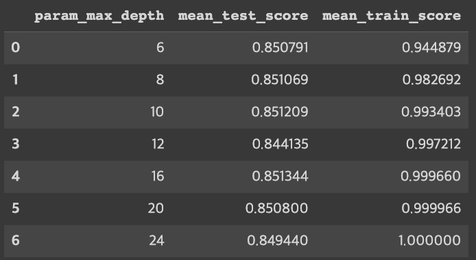
print('최고 평균 정확도: {0:.4f}, 최적 하이퍼 매개변수: {1}'.format(grid_cv.best_score_, grid_cv.best_params_))
최고 평균 정확도: 0.8513, 최적 하이퍼 매개변수: {'max_depth': 16}
max_depth와 함께 min_sample_split을 조정하면서 최고의 평균 정확도 확인해 보자
params = {
    'max_depth' : [8, 16, 20],
    'min_samples_split' : [8, 16, 24]
}

grid_cv = GridSearchCV(dt_HAR, param_grid = params, scoring = 'accuracy', cv = 5, return_train_score = True)
grid_cv.fit(X_train, Y_train)
GridSearchCV(cv=5, estimator=DecisionTreeClassifier(random_state=156),
             param_grid={'max_depth': [8, 16, 20],
                         'min_samples_split': [8, 16, 24]},
             return_train_score=True, scoring='accuracy')

cv_results_df = pd.DataFrame(grid_cv.cv_results_)

cv_results_df[['param_max_depth', 'param_min_samples_split', 'mean_test_score', 'mean_train_score']]
print('최고 평균 정확도: {0:.4f}, 최적 하이퍼 매개변수: {1}'.format(grid_cv.best_score_, grid_cv.best_params_))
최고 평균 정확도: 0.8549, 최적 하이퍼 매개변수: {'max_depth': 8, 'min_samples_split': 16}
최적모델(grid_cv.best_estimator_)을 사용하여 테스트 데이터에 대한 예측을 수행해 보자.
best_dt_HAR = grid_cv.best_estimator_
best_Y_predict = best_dt_HAR.predict(X_test)
best_accuracy = accuracy_score(Y_test, best_Y_predict)

print('best 결정 트리 예측 정확도: {0:.4f}'.format(best_accuracy))
best 결정 트리 예측 정확도: 0.8717
결정 트리 모델은 feature_importances_ 속성을 사용하여 중요도가 높은 10개 피처를 찾아 그래프로 나타내보자.
import seaborn as sns
import matplotlib.pyplot as plt

feature_importance_values = best_dt_HAR.feature_importances_
feature_importance_values_s = pd.Series(feature_importance_values, index = X_train.columns)
feature_top10 = feature_importance_values_s.sort_values(ascending = False)[:10]

plt.figure(figsize = (10, 5))
plt.title('Feature Top 10')
sns.barplot(x = feature_top10, y = feature_top10.index)
plt.show()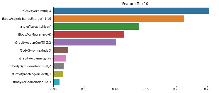
결과 시각화
결정 트리 모델의 트리 구조를 그림으로 시각화하기
!pip install graphviz
Looking in indexes: https://pypi.org/simple, https://us-python.pkg.dev/colab-wheels/public/simple/
Requirement already satisfied: graphviz in /usr/local/lib/python3.8/dist-packages (0.10.1)

from sklearn.tree import export_graphviz

#export_graphviz()의 호출 결과로 out_file로 지정된 tree.dot 파일 생성 export_graphviz(best_dt_HAR, out_file = "tree.dot", class_names = label_name, feature_names = feature_name, impurity = True, filled = Ture)

import graphviz

#위에서 생성된 tree.dot 파일을 Graphviz가 읽어서 시각화
with open("/tree.dot") as f:
    dot_graph = f.read()

graphviz.Source(dot_graph)
'Python > 데이터 과학 기반의 파이썬 빅데이터 분석(한빛 아카데미)' 카테고리의 다른 글
| 데이터 과학 기반의 파이썬 빅데이터 분석 Chapter13 텍스트 마이닝 (2) | 2023.01.11 |
|---|---|
| 데이터 과학 기반의 파이썬 빅데이터 분석 Chapter12 군집분석 (0) | 2023.01.10 |
| 데이터 과학 기반의 파이썬 빅데이터 분석 Chapter10 회귀 분석 (0) | 2023.01.09 |
| 데이터 과학 기반의 파이썬 빅데이터 분석 Chapter09 지리 정보 분석 (0) | 2023.01.09 |
| 데이터 과학 기반의 파이썬 빅데이터 분석 Chapter08 텍스트 빈도 분석 (0) | 2023.01.08 |


