EDA
!wget 'https://bit.ly/3i4n1QB'
import zipfile
with zipfile.ZipFile('3i4n1QB', 'r') as existing_zip:
existing_zip.extractall('data')
import pandas as pd
import numpy as np
import matplotlib
import matplotlib.pyplot as plt
import seaborn as sns
# read_csv() 매서드로 train.csv , test.csv파일을 df class 로 불러오세요.
train = pd.read_csv('data/train.csv')
test = pd.read_csv('data/test.csv')
# info() 매서드로 데이터의 정보를 확인하세요.
train.info()
# shape 어트리뷰트로 행, 열을 파악하세요.
train.shape
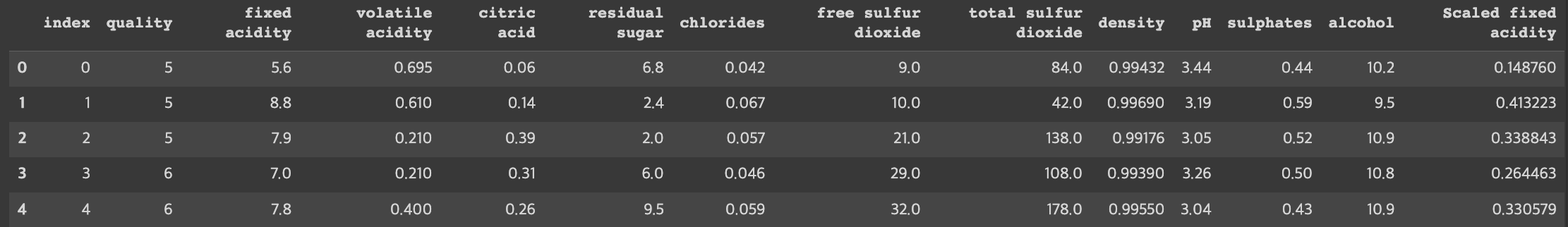
# head() 매서드로 데이터의 각 컬럼의 정보를 조사하세요.
train.head()
# isnull() 매서드로 결측치 존재여부를 확인하세요.
train.isnull()
# sum() 매서드로 결측치의 갯수를 출력하세요.
train.isnull().sum()
# copy() 매서드로 학습 데이터의 복사본을 생성하세요.
traindata = train.copy()
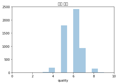
# 타깃 변수(와인 품질) 분포 시각화
sns.distplot(traindata['quality'], kde=False, bins=10)
plt.axis([0, 10, 0, 2500]) # [x 축 최솟값, x 축 최댓값, y 축 최솟값, y 축 최댓값]
plt.title("와인 품질") # 그래프 제목 지정
plt.show() # 그래프 그리기
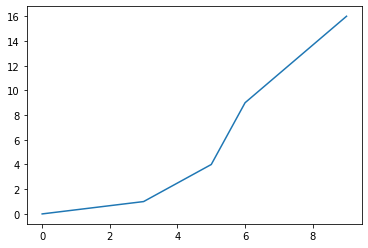
# x축 지점의 값들로 정할 리스트를 생성합니다.
x_values = [0, 3, 5, 6, 9]
# y축 지점의 값들
y_values = [0, 1, 4, 9, 16]
# line 그래프를 그린 후 화면에 보여줍니다.
plt.plot(x_values, y_values)
plt.show()
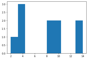
# 변수 분포를 갖는 리스트를 생성합니다.
a = [2,4,4,4,8,8,10,10,14,14]
# line 그래프를 그린 후 화면에 보여줍니다.
plt.hist(a)
plt.show()
--2023-02-27 02:56:06-- https://bit.ly/3i4n1QB
Resolving bit.ly (bit.ly)... 67.199.248.10, 67.199.248.11
Connecting to bit.ly (bit.ly)|67.199.248.10|:443... connected.
HTTP request sent, awaiting response... 301 Moved Permanently
Location: https://drive.google.com/uc?export=download&id=1emLrrpFWT8dCoj5BJb12-5QMG2-nruUw [following]
--2023-02-27 02:56:06-- https://drive.google.com/uc?export=download&id=1emLrrpFWT8dCoj5BJb12-5QMG2-nruUw
Resolving drive.google.com (drive.google.com)... 172.253.62.113, 172.253.62.101, 172.253.62.138, ...
Connecting to drive.google.com (drive.google.com)|172.253.62.113|:443... connected.
HTTP request sent, awaiting response... 303 See Other
Location: https://doc-10-10-docs.googleusercontent.com/docs/securesc/ha0ro937gcuc7l7deffksulhg5h7mbp1/02r8kv1khrr3vqviirnomeqplrehrkq9/1677466500000/17946651057176172524/*/1emLrrpFWT8dCoj5BJb12-5QMG2-nruUw?e=download&uuid=fb8a967e-5b77-45ed-87da-e57de99e9672 [following]
Warning: wildcards not supported in HTTP.
--2023-02-27 02:56:07-- https://doc-10-10-docs.googleusercontent.com/docs/securesc/ha0ro937gcuc7l7deffksulhg5h7mbp1/02r8kv1khrr3vqviirnomeqplrehrkq9/1677466500000/17946651057176172524/*/1emLrrpFWT8dCoj5BJb12-5QMG2-nruUw?e=download&uuid=fb8a967e-5b77-45ed-87da-e57de99e9672
Resolving doc-10-10-docs.googleusercontent.com (doc-10-10-docs.googleusercontent.com)... 142.251.16.132, 2607:f8b0:4004:c17::84
Connecting to doc-10-10-docs.googleusercontent.com (doc-10-10-docs.googleusercontent.com)|142.251.16.132|:443... connected.
HTTP request sent, awaiting response... 200 OK
Length: 137694 (134K) [application/zip]
Saving to: ‘3i4n1QB.3’
3i4n1QB.3 100%[===================>] 134.47K --.-KB/s in 0.002s
2023-02-27 02:56:07 (80.5 MB/s) - ‘3i4n1QB.3’ saved [137694/137694]
<class 'pandas.core.frame.DataFrame'>
RangeIndex: 5497 entries, 0 to 5496
Data columns (total 14 columns):
# Column Non-Null Count Dtype
--- ------ -------------- -----
0 index 5497 non-null int64
1 quality 5497 non-null int64
2 fixed acidity 5497 non-null float64
3 volatile acidity 5497 non-null float64
4 citric acid 5497 non-null float64
5 residual sugar 5497 non-null float64
6 chlorides 5497 non-null float64
7 free sulfur dioxide 5497 non-null float64
8 total sulfur dioxide 5497 non-null float64
9 density 5497 non-null float64
10 pH 5497 non-null float64
11 sulphates 5497 non-null float64
12 alcohol 5497 non-null float64
13 type 5497 non-null object
dtypes: float64(11), int64(2), object(1)
memory usage: 601.4+ KB
/usr/local/lib/python3.8/dist-packages/seaborn/distributions.py:2619: FutureWarning: `distplot` is a deprecated function and will be removed in a future version. Please adapt your code to use either `displot` (a figure-level function with similar flexibility) or `histplot` (an axes-level function for histograms).
warnings.warn(msg, FutureWarning)
/usr/local/lib/python3.8/dist-packages/IPython/core/pylabtools.py:128: UserWarning: Glyph 50752 (\N{HANGUL SYLLABLE WA}) missing from current font.
fig.canvas.print_figure(bytes_io, **kw)
/usr/local/lib/python3.8/dist-packages/IPython/core/pylabtools.py:128: UserWarning: Glyph 51064 (\N{HANGUL SYLLABLE IN}) missing from current font.
fig.canvas.print_figure(bytes_io, **kw)
/usr/local/lib/python3.8/dist-packages/IPython/core/pylabtools.py:128: UserWarning: Glyph 54408 (\N{HANGUL SYLLABLE PUM}) missing from current font.
fig.canvas.print_figure(bytes_io, **kw)
/usr/local/lib/python3.8/dist-packages/IPython/core/pylabtools.py:128: UserWarning: Glyph 51656 (\N{HANGUL SYLLABLE JIL}) missing from current font.
fig.canvas.print_figure(bytes_io, **kw)
전처리
# boxplot() 매서드로 'fixed acidity' 피쳐의 이상치를 확인하는 코드를 아래에 작성하세요.
sns.boxplot(data=train['fixed acidity'])

# "fixed acidity"가 25%인 값을 "quantile_25" 라는 변수에 만들어 주세요
quantile_25 = np.quantile(train['fixed acidity'], 0.25)

# "fixed acidity"가 75%인 값을 "quantile_75" 라는 변수에 만들어 주세요
quantile_75 = np.quantile(train['fixed acidity'],0.75)

# quantile_75와 quantile_25의 차이를 "IQR"이라는 변수에 만들어 주세요
IQR = quantile_75 - quantile_25

# quantile_25보다 1.5 * IQR 작은 값을 "minimum"이라는 변수에 만들어 주세요
minimum = quantile_25 - 1.5 * IQR

# quantile_75보다 1.5 * IQR 큰 값을 "maximum"이라는 변수에 만들어 주세요
maximum = quantile_75 + 1.5 * IQR

# "fixed acidity"가 minimum보다 크고, maximum보다 작은 값들만 "train2"에 저장해 주세요
train2 = train[(minimum <= train['fixed acidity']) & (train['fixed acidity'] <= maximum)]

# train2.shape를 통해서, 총 몇개의 행이 되었는지 확인해보세요.
train2.shape

# 몇개의 이상치가 있는지도 계산해보세요.
# 294개의 이상치를 발견해 제거했습니다.
train.shape[0] - train2.shape[0]

# describe를 통해 "fixed acidity"의 데이터의 분포가 어떻게 생겼는지 짐작해보세요
train.describe()

# seaborn의 displot을 통해 "fixed acidity"의 distplot을 그려보세요.
sns.distplot(train['fixed acidity'])

# MinMaxScaler를 "scaler"라는 변수에 지정해주세요.
scaler = MinMaxScaler()

# "scaler"를 학습시켜주세요.
scaler.fit(train[['fixed acidity']])

# "scaler"를 통해 train과 test의 "fixed acidity"를 바꾸어 "Scaled fixed acidity"라는 column에 저장해주세요.
train['Scaled fixed acidity'] = scaler.transform(train[['fixed acidity']])
test['Scaled fixed acidity'] = scaler.transform(test[['fixed acidity']])

# seaborn의 displot을 통해 "Scaled fixed acidity"의 distplot을 그려보세요
sns.distplot(train['Scaled fixed acidity'])

# "OneHotEncoder"를 "encoder"라는 변수에 저장해보세요.
encoder = OneHotEncoder()

# "encoder"를 사용해 train의 "type" 피쳐를 학습시켜보세요.
encoder.fit(train[['type']])

# "encoder"를 사용해 train의 "type"피쳐를 변환해 "onehot"이라는 변수에, test의 "type"피쳐를 변환해 "onehot2"라는 변수에 저장해보세요.
onehot = encoder.transform(train[['type']])
onehot2 = encoder.transform(test[['type']])
onehot

# "onehot", "onehot2" 라는 변수를 array 형태로 변환해 보세요.
onehot = onehot.toarray()
onehot2 = onehot2.toarray()
onehot

# "onehot","onethot2"라는 변수를 DataFrame 형태로 변환해 보세요
onehot = pd.DataFrame(onehot)
onehot2 = pd.DataFrame(onehot2)
onehot.head()

# encoder의 "get_feature_names()"를 사용해 column 이름을 바꿔보세요
onehot.columns = encoder.get_feature_names()
onehot2.columns = encoder.get_feature_names()
onehot.head()

# onehot, onehot2를 원본데이터인 train,test에 병합시켜보세요.
onehot = pd.concat([train, onehot], axis = 1)
onehot.head()

# train과 test의 "type" 변수를 제거해주세요.
train = train.drop(columns = ['type'])
test = test.drop(columns = ['type'])
train.head()

/usr/local/lib/python3.8/dist-packages/seaborn/distributions.py:2619: FutureWarning: `distplot` is a deprecated function and will be removed in a future version. Please adapt your code to use either `displot` (a figure-level function with similar flexibility) or `histplot` (an axes-level function for histograms).
  warnings.warn(msg, FutureWarning)
/usr/local/lib/python3.8/dist-packages/sklearn/utils/deprecation.py:87: FutureWarning: Function get_feature_names is deprecated; get_feature_names is deprecated in 1.0 and will be removed in 1.2. Please use get_feature_names_out instead.
  warnings.warn(msg, category=FutureWarning)

모델링
# 랜덤포레스트 분류 모형을 불러오세요.
from sklearn.ensemble import RandomForestClassifier

# 랜덤포레스트 분류 모형을 "random_forest"라는 변수에 저장하세요.
random_forest = RandomForestClassifier()
random_forest

# "X"라는 변수에 train의 "quality" 피쳐를 제거하고 저장하세요.
X = train.drop(columns = ['quality'])

# "y"라는 변수에 정답인 train의 "quality" 피쳐를 저장하세요.
y = train['quality']

# "random_classifier"를 X와 y를 이용해 학습시켜보세요.
random_forest.fit(X,y)

# sklearn에 model_selection 부분 속 KFold를 불러와보세요.
from sklearn.model_selection import KFold

# KFold에 n_splits = 5, shuffle = True, random_state = 0이라는 인자를 추가해 "kf"라는 변수에 저장해보세요.
kf = KFold(n_splits = 5, shuffle = True, random_state = 0)

# 반복문을 통해서 1번부터 5번까지의 데이터에 접근해보세요.

for train_idx, valid_idx in kf.split(train) :
  train_data = train.iloc[train_idx]
  valid_data = train.iloc[valid_idx]

import matplotlib.pyplot as plt


kf = KFold(n_splits = 5, shuffle = False, random_state = 0)
train_idx_store = []
valid_idx_store = []

i = 1
for train_idx, valid_idx in kf.split(train) :
  plt.scatter(valid_idx, [i for x in range(len(valid_idx))], alpha = 0.1)
  i += 1
plt.show()

# "X"라는 변수에 train의 "index"와 "quality"를 제외하고 지정해 주세요
# "y"라는 변수에는 "quality"를 지정해 주세요
X = train.drop(columns = ['index','quality'])
y = train['quality']

# "kf"라는 변수에 KFold를 지정해 줍시다.
# n_splits는 5, shuffle은 True, random_state는 0으로 설정해주세요
kf = KFold(n_splits = 5, shuffle = True, random_state = 0)

# "model"이라는 변수에 RandomForestClassifier를 지정해 줍시다.
# valid_scores라는 빈 리스트를 하나 만들어줍시다.
# test_predictions라는 빈 리스트를 하나 만들어 줍시다.
model = RandomForestClassifier(random_state = 0)
valid_scores = []
test_predictions = []

# 지난 시간에 다루었던 kf.split()을 활용해, 반복문으로 X_tr, y_tr, X_val, y_val을 설정해봅시다.
for train_idx, valid_idx in kf.split(X,y) :
  X_tr = X.iloc[train_idx]
  y_tr = y.iloc[train_idx]

  X_val = X.iloc[valid_idx]
  y_val = y.iloc[valid_idx]

# 앞의 문제에 이어서 반복문 속에서 model.fit(X_tr, y_tr)을 활용해 모델을 학습해봅시다
for train_idx, valid_idx in kf.split(X,y) :
  X_tr = X.iloc[train_idx]
  y_tr = y.iloc[train_idx]

  X_val = X.iloc[valid_idx]
  y_val = y.iloc[valid_idx]

  model.fit(X_tr, y_tr)

# 앞의 문제에 이어서 반복문 속에서 "valid_prediction"이라는 변수에 model.predict(X_val)의 결과를 저장해 봅시다.
for train_idx, valid_idx in kf.split(X,y) :
  X_tr = X.iloc[train_idx]
  y_tr = y.iloc[train_idx]

  X_val = X.iloc[valid_idx]
  y_val = y.iloc[valid_idx]

  model.fit(X_tr, y_tr)

  valid_prediction = model.predict(X_val)

# 앞의 문제에 이어서 반복문 속에서 accuracy_score를 이용해, 모델이 어느정도의 예측 성능이 나올지 확인해봅시다.
# 그리고 "valid_prediction"의 점수를 scores에 저장 해봅시다.
# 반복문에서 빠져나온 후에 np.mean()을 활용해 평균 점수를 예측해봅시다.
for train_idx, valid_idx in kf.split(X,y) :
  X_tr = X.iloc[train_idx]
  y_tr = y.iloc[train_idx]

  X_val = X.iloc[valid_idx]
  y_val = y.iloc[valid_idx]

  model.fit(X_tr, y_tr)

  valid_prediction = model.predict(X_val)
  score = metrics.accuracy_score(y_val, valid_prediction)
  valid_scores.append(score)
  print(score)
print('평균 점수 : ', np.mean(valid_scores))

# 이제 어느정도의 성능이 나올지 알게 되었으니, 반복문 속에서 test를 예측해 "test_prediction"이라는 변수에 지정해봅시다.
# test_prediction을 지정했다면, "test_precitions"라는 빈 리스트에 넣어줍시다.

for train_idx, valid_idx in kf.split(X,y) :
  X_tr = X.iloc[train_idx]
  y_tr = y.iloc[train_idx]

  X_val = X.iloc[valid_idx]
  y_val = y.iloc[valid_idx]

  model.fit(X_tr, y_tr)

  test_prediction = model.predict(test.drop(columns = ['index']))
  test_predictions.append(test_prediction)

# 이제 결과 값을 만들어 보겠습니다.
# "test_precitions"를 Data Frame으로 만들어주세요.
test_predictions = pd.DataFrame(test_predictions)
test_predictions

# DF.mode()를 활용해 열별 최빈값을 확인하고, "test_prediction"이라는 변수에 지정해봅시다.
# "test_prediction"의 첫 행을 최종 결과값으로 사용합시다.
test_prediction = test_predictions.mode()
test_prediction = test_predictions.values[0]
test_prediction

# data의 sample_submission 파일을 불러와 "quality"라는 변수에 "test_precition"을 저장해줍시다.
# 그 이후에는, "data/submission_KFOLD.csv"에 저장하고, 제출해봅시다.
sample_submission = pd.read_csv('data/sample_submission.csv')
sample_submission['quality'] = test_prediction
sample_submission.to_csv('data/submission_KFOLD.csv', index=False)

0.6854545454545454
0.68
0.654231119199272
0.6624203821656051
0.6642402183803457
평균 점수 :  0.6692692530399535

튜닝
# bayesian-optimization을 설치해보세요.
!pip install bayesian-optimization

# bayes_opt 패키지에서 BayesianOptimization을 불러와보세요.
from bayes_opt import BayesianOptimization
from sklearn.model_selection import train_test_split

# X에 학습할 데이터를, y에 목표 변수를 저장해주세요
X = train.drop(columns = ['index', 'quality'])
y = train['quality']

# 랜덤포레스트의 하이퍼 파라미터의 범위를 dictionary 형태로 지정해주세요
## Key는 랜덤포레스트의 hyperparameter이름이고, value는 탐색할 범위 입니다.
rf_parameter_bounds = {
                      'max_depth' : (1,3), # 나무의 깊이
                      'n_estimators' : (30,100),
                      }

# 함수를 만들어주겠습니다.
# 함수의 구성은 다음과 같습니다.
# 1. 함수에 들어가는 인자 = 위에서 만든 함수의 key값들
# 2. 함수 속 인자를 통해 받아와 새롭게 하이퍼파라미터 딕셔너리 생성
# 3. 그 딕셔너리를 바탕으로 모델 생성
# 4. train_test_split을 통해 데이터 train-valid 나누기
# 5 .모델 학습
# 6. 모델 성능 측정
# 7. 모델의 점수 반환

def rf_bo(max_depth, n_estimators):
  rf_params = {
              'max_depth' : int(round(max_depth)),
               'n_estimators' : int(round(n_estimators)),
              }
  rf = RandomForestClassifier(**rf_params)

  X_train, X_valid, y_train, y_valid = train_test_split(X,y,test_size = 0.2, )

  rf.fit(X_train,y_train)
  score = metrics.accuracy_score(y_valid, rf.predict(X_valid))
  return score

# 이제 Bayesian Optimization을 사용할 준비가 끝났습니다.
# "BO_rf"라는 변수에 Bayesian Optmization을 저장해보세요
BO_rf = BayesianOptimization(f = rf_bo, pbounds = rf_parameter_bounds,random_state = 0)

# Bayesian Optimization을 실행해보세요
BO_rf.maximize(init_points = 5, n_iter = 5)

# 하이퍼파라미터의 결과값을 불러와 "max_params"라는 변수에 저장해보세요
max_params = BO_rf.max['params']

max_params['max_depth'] = int(max_params['max_depth'])
max_params['n_estimators'] = int(max_params['n_estimators'])
print(max_params)

# Bayesian Optimization의 결과를 "BO_tuend_rf"라는 변수에 저장해보세요
BO_tuend_rf = RandomForestClassifier(**max_params)

Looking in indexes: https://pypi.org/simple, https://us-python.pkg.dev/colab-wheels/public/simple/
Requirement already satisfied: bayesian-optimization in /usr/local/lib/python3.8/dist-packages (1.4.2)
Requirement already satisfied: numpy>=1.9.0 in /usr/local/lib/python3.8/dist-packages (from bayesian-optimization) (1.22.4)
Requirement already satisfied: scikit-learn>=0.18.0 in /usr/local/lib/python3.8/dist-packages (from bayesian-optimization) (1.0.2)
Requirement already satisfied: scipy>=1.0.0 in /usr/local/lib/python3.8/dist-packages (from bayesian-optimization) (1.7.3)
Requirement already satisfied: colorama>=0.4.6 in /usr/local/lib/python3.8/dist-packages (from bayesian-optimization) (0.4.6)
Requirement already satisfied: joblib>=0.11 in /usr/local/lib/python3.8/dist-packages (from scikit-learn>=0.18.0->bayesian-optimization) (1.2.0)
Requirement already satisfied: threadpoolctl>=2.0.0 in /usr/local/lib/python3.8/dist-packages (from scikit-learn>=0.18.0->bayesian-optimization) (3.1.0)
|   iter    |  target   | max_depth | n_esti... |
-------------------------------------------------
| 1         | 0.5391    | 2.098     | 80.06     |
| 2         | 0.5373    | 2.206     | 68.14     |
| 3         | 0.5436    | 1.847     | 75.21     |
| 4         | 0.5445    | 1.875     | 92.42     |
| 5         | 0.5455    | 2.927     | 56.84     |
| 6         | 0.4427    | 1.018     | 48.01     |
| 7         | 0.5227    | 2.847     | 99.74     |
| 8         | 0.4645    | 1.027     | 61.91     |
| 9         | 0.5427    | 3.0       | 55.47     |
| 10        | 0.5473    | 1.962     | 87.78     |
=================================================
{'max_depth': 1, 'n_estimators': 87}