데이터 다운로드
# 데이터 다운로드 링크로 데이터를 코랩에 불러옵니다.
!wget 'https://bit.ly/3i4n1QB'

import zipfile
with zipfile.ZipFile('3i4n1QB', 'r') as existing_zip:
    existing_zip.extractall('data')

# 라이브러리 및 데이터 불러오기
import pandas as pd
from sklearn.preprocessing import MinMaxScaler, OneHotEncoder, PolynomialFeatures
from lightgbm import LGBMClassifier
from xgboost import XGBClassifier
from sklearn.ensemble import RandomForestClassifier
from sklearn.ensemble import VotingClassifier

from sklearn.model_selection import KFold, train_test_split
from sklearn.metrics import accuracy_score
import numpy as np
import seaborn as sns
import matplotlib.pyplot as plt

# VIF기능을 제공하는 라이브러리 불러오기
from statsmodels.stats.outliers_influence import variance_inflation_factor

# sklearn 의 MinMaxScaler 라이브러리 불러오기
from sklearn.preprocessing import MinMaxScaler

# PCA 라이브러리 호출
from sklearn.decomposition import PCA

# 데이터를 불러와 학습시킬 준비하기
train = pd.read_csv('data/train.csv')
test = pd.read_csv('data/test.csv')

train.drop('index',axis = 1, inplace = True)
test.drop('index',axis = 1, inplace = True)

train = pd.get_dummies(train)
test = pd.get_dummies(test)
EDA
# "data"라는 변수에 train의 "fixed acidity"부터 "chlorides"까지의 변수를 저장해주세요
data = train.loc[:, 'fixed acidity' : 'chlorides']

# data의 pairplot을 그려보세요
sns.pairplot(data)
<seaborn.axisgrid.PairGrid at 0x7f2ea648d9a0>
# "data"라는 변수에 train의 "fixed acidity"부터 "chlorides"까지의 변수를 저장해주세요
data = train['fixed acidity']

# data의 pairplot을 그려보세요
sns.distplot(data,bins = 100)
/usr/local/lib/python3.8/dist-packages/seaborn/distributions.py:2619: FutureWarning: `distplot` is a deprecated function and will be removed in a future version. Please adapt your code to use either `displot` (a figure-level function with similar flexibility) or `histplot` (an axes-level function for histograms).
  warnings.warn(msg, FutureWarning)
<matplotlib.axes._subplots.AxesSubplot at 0x7f2e88e03310>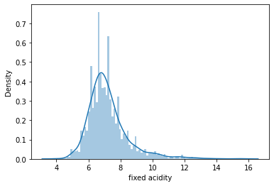
# 히트맵 그래프를 그릴 변수 지정 (train.corr() )
# corr() 함수는 데이터의 변수간의 상관도를 출력하는 함수 입니다.
data = train.corr()

# seaborn 의 heatmap 함수를 이용해 히트맵 그래프를 그립니다.
sns.heatmap(data)
<matplotlib.axes._subplots.AxesSubplot at 0x7f2e84f567c0>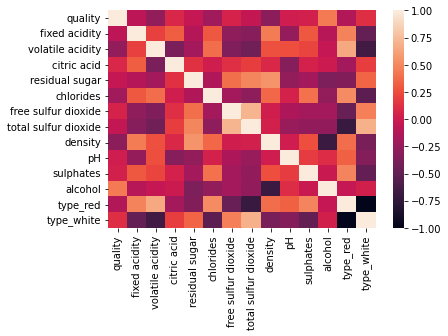
# Scatter Plot을 그릴 변수 지정 (
x_data = train['residual sugar']
y_data = train['density']

# seaborn 의 scatterplot함수를 이용해 그래프를 그립니다.
sns.scatterplot(x = x_data, y = y_data )
<matplotlib.axes._subplots.AxesSubplot at 0x7f2e84f5dee0>
전처리
# train 데이터의 VIF 계수 출력
vif = pd.DataFrame()
vif["VIF Factor"] = [variance_inflation_factor(train.values, i) for i in range(train.shape[1])]
vif["features"] = train.columns

# MinMaxScaler를 통해 변수 변환
scaler = MinMaxScaler()
scaler.fit(train) # fit 함수를 이용해  scaler 학습
train_scale = scaler.transform(train)# "scaler"를 통해 train의 수치들을 변환 시키고 train_scale에 저장 해 주세요.

# Sclaer 를 통해 변환된 데이터의 VIF 확인
new_train_df =  pd.DataFrame(train_scale)
new_train_df.columns = train.columns
vif = pd.DataFrame()
vif["VIF Factor"] = [variance_inflation_factor(new_train_df.values, i) for i in range(new_train_df.shape[1])]
vif["features"] = new_train_df.columns

from sklearn.datasets import load_iris
import pandas as pd

# 사이킷런 내장 데이터 셋 API 호출
iris = load_iris()

# DataFrame으로 변환
df = pd.DataFrame(iris.data)
df.columns =  ['sepal_length','sepal_width','petal_length','petal_width']
df['target']=iris.target
df.head(3)

#setosa는 빨간색, versicolor는 노란색, virginica는 파란색
color=['r', 'y', 'b']

# setosa의 target 값은 0, versicolor는 1, virginica는 2.
# 각 target 별로 다른 색으로 scatter plot
for i, c in enumerate(color):
    x_axis_data = df[df['target']==i]['sepal_length']
    y_axis_data = df[df['target']==i]['sepal_width']
    plt.scatter(x_axis_data, y_axis_data,color = c,label=iris.target_names[i])

plt.legend()
plt.xlabel('sepal length')
plt.ylabel('sepal width')
plt.show()

# Target 값을 제외한 모든 속성 값을 MinMaxScaler를 이용하여 변환
# 'sepal_length','sepal_width','petal_length','petal_width'
df_features = df[['sepal_length','sepal_width','petal_length','petal_width']]
df_scaler = MinMaxScaler().fit_transform(df_features)

# PCA를 이용하여 4차원 변수를 2차원으로 변환
pca = PCA(n_components=2)

#fit( )과 transform( ) 을 호출하여 PCA 변환 / 데이터 반환
pca.fit(df_scaler)
df_pca = pca.transform(df_scaler)
print(df_pca.shape)

# PCA 변환된 데이터의 컬럼명을 각각 PCA_1, PCA_2로 지정
df_pca = pd.DataFrame(df_pca)
df_pca.columns = ['PCA_1','PCA_2']
df_pca['target']=df.target
df_pca.head(3)

#setosa는 빨간색, versicolor는 노란색, virginica는 파란색
color=['r', 'y', 'b']

# setosa의 target 값은 0, versicolor는 1, virginica는 2.
# 각 target 별로 다른 색으로 scatter plot

for i, c in enumerate(color):
    x_axis_data = df_pca[df_pca['target']==i]['PCA_1']
    y_axis_data = df_pca[df_pca['target']==i]['PCA_2']
    plt.scatter(x_axis_data, y_axis_data, color = c,label=iris.target_names[i])

plt.legend()
plt.xlabel('PCA_1')
plt.ylabel('PCA_2')
plt.show()

 # train 데이터의 alcohol 변수를 구간이 5개인 범주형 변수로 변환
 train['alcohol'] = pd.cut(train.alcohol, 5,labels=False)

 from sklearn.tree import DecisionTreeClassifier

# train 데이터를 PolynomialFeatures 를 이용하여 변환
poly_features = PolynomialFeatures(degree=2) # 차원은 2로 설정

# 와인 품질 기준인 quality 변수를 제외한 나머지 변수를 포함한 데이터 변환.
df = train.drop('quality',axis = 1)
df_poly = poly_features.fit_transform(df) # fit_transform 메소드를 통해 데이터 변환
df_poly = pd.DataFrame(df_poly) # PolynomialFeatures로 변환 된 데이터를 데이터 프레임 형태로 변환

# DecisionTreeClassifier 모델을 변환된 train 데이터로 학습
from sklearn.tree import DecisionTreeClassifier
model = DecisionTreeClassifier()
model.fit(df_poly,train['quality'])

# test 데이터 변환
poly_features = PolynomialFeatures(degree=2) # 차원은 2로 설정
test_poly = poly_features.fit_transform(test) # fit_transform 메소드를 통해 데이터 변환
test_poly = pd.DataFrame(test_poly) # PolynomialFeatures로 변환 된 데이터를 데이터 프레임 형태로 변환

# 결괏값 추론
pred = model.predict(test_poly)

# 정답 파일 생성
submission = pd.read_csv('data/sample_submission.csv')
submission['quality'] = pred
submission.to_csv('poly.csv',index = False)
모델링 및 튜닝
Random forest 튜닝
# X에 학습할 데이터를, y에 목표 변수를 저장해주세요
X = train.drop(columns = ['index', 'quality'])
y = train['quality']

# 랜덤포레스트의 하이퍼 파라미터의 범위를 dictionary 형태로 지정해주세요
## Key는 랜덤포레스트의 hyperparameter이름이고, value는 탐색할 범위 입니다.
rf_parameter_bounds = {
                      'max_depth' : (1,3), # 나무의 깊이
                      'n_estimators' : (30,100),
                      }

# 함수를 만들어주겠습니다.

# 함수의 구성은 다음과 같습니다.
# 1. 함수에 들어가는 인자 = 위에서 만든 함수의 key값들
# 2. 함수 속 인자를 통해 받아와 새롭게 하이퍼파라미터 딕셔너리 생성
# 3. 그 딕셔너리를 바탕으로 모델 생성
# 4. train_test_split을 통해 데이터 train-valid 나누기
# 5 .모델 학습
# 6. 모델 성능 측정
# 7. 모델의 점수 반환
def rf_bo(max_depth, n_estimators):
  rf_params = {
              'max_depth' : int(round(max_depth)),
               'n_estimators' : int(round(n_estimators)),
              }
  rf = RandomForestClassifier(**rf_params)
  X_train, X_valid, y_train, y_valid = train_test_split(X,y,test_size = 0.2, )
  rf.fit(X_train,y_train)
  score = accuracy_score(y_valid, rf.predict(X_valid))
  return score

# 이제 Bayesian Optimization을 사용할 준비가 끝났습니다.
# "BO_rf"라는 변수에 Bayesian Optmization을 저장해보세요
BO_rf = BayesianOptimization(f = rf_bo, pbounds = rf_parameter_bounds,random_state = 0)

# Bayesian Optimization을 실행해보세요
BO_rf.maximize(init_points = 5, n_iter = 5)
xgb 튜닝
# X에 학습할 데이터를, y에 목표 변수를 저장해주세요
X = train.drop(columns = ['index', 'quality'])
y = train['quality']

# XGBoost의 하이퍼 파라미터의 범위를 dictionary 형태로 지정해주세요
## Key는 XGBoost hyperparameter이름이고, value는 탐색할 범위 입니다.
xgb_parameter_bounds = {
                      'gamma' : (0,10),
                      'max_depth' : (1,3),
                      'subsample' : (0.5,1)
                      }

# 함수를 만들어주겠습니다.
# 함수의 구성은 다음과 같습니다.
# 1. 함수에 들어가는 인자 = 위에서 만든 함수의 key값들
# 2. 함수 속 인자를 통해 받아와 새롭게 하이퍼파라미터 딕셔너리 생성
# 3. 그 딕셔너리를 바탕으로 모델 생성
# 4. train_test_split을 통해 데이터 train-valid 나누기
# 5 .모델 학습
# 6. 모델 성능 측정
# 7. 모델의 점수 반환
def xgb_bo(gamma,max_depth, subsample):
  xgb_params = {
              'gamma' : int(round(gamma)),
              'max_depth' : int(round(max_depth)),
               'subsample' : int(round(subsample)),
              }
  xgb = XGBClassifier(**xgb_params)
  X_train, X_valid, y_train, y_valid = train_test_split(X,y,test_size = 0.2, )
  xgb.fit(X_train,y_train)
  score = accuracy_score(y_valid, xgb.predict(X_valid))
  return score

# 이제 Bayesian Optimization을 사용할 준비가 끝났습니다.
# "BO_xgb"라는 변수에 Bayesian Optmization을 저장해보세요
BO_xgb = BayesianOptimization(f = xgb_bo, pbounds = xgb_parameter_bounds,random_state = 0)

# Bayesian Optimization을 실행해보세요
BO_xgb.maximize(init_points = 5, n_iter = 5)
LGBM 튜닝
# X에 학습할 데이터를, y에 목표 변수를 저장해주세요
X = train.drop(columns = ['index', 'quality'])
y = train['quality']


# LGBM의 하이퍼 파라미터의 범위를 dictionary 형태로 지정해주세요
## Key는 LGBM hyperparameter이름이고, value는 탐색할 범위 입니다.
lgbm_parameter_bounds = {
                      'n_estimators' : (30,100),
                      'max_depth' : (1,3), # 나무의 깊이
                      'subsample' : (0.5,1)
                      }

# 함수를 만들어주겠습니다.

# 함수의 구성은 다음과 같습니다.
# 1. 함수에 들어가는 인자 = 위에서 만든 함수의 key값들
# 2. 함수 속 인자를 통해 받아와 새롭게 하이퍼파라미터 딕셔너리 생성
# 3. 그 딕셔너리를 바탕으로 모델 생성
# 4. train_test_split을 통해 데이터 train-valid 나누기
# 5 .모델 학습
# 6. 모델 성능 측정
# 7. 모델의 점수 반환
def lgbm_bo(n_estimators,max_depth, subsample):
  lgbm_params = {
              'n_estimators' : int(round(n_estimators)),
              'max_depth' : int(round(max_depth)),
               'subsample' : int(round(subsample)),
              }
  lgbm = LGBMClassifier(**lgbm_params)

  X_train, X_valid, y_train, y_valid = train_test_split(X,y,test_size = 0.2, )
  lgbm.fit(X_train,y_train)
  score = accuracy_score(y_valid, lgbm.predict(X_valid))

  return score

# 이제 Bayesian Optimization을 사용할 준비가 끝났습니다.
# "BO_lgbm"라는 변수에 Bayesian Optmization을 저장해보세요
BO_lgbm = BayesianOptimization(f = lgbm_bo, pbounds = lgbm_parameter_bounds,random_state = 0)

# Bayesian Optimization을 실행해보세요
BO_lgbm.maximize(init_points = 5, n_iter = 5)
voting classifier 정의 및 예측
X = train_one.drop('quality',axis= 1)
y = train_one['quality']

# 모델 정의 (튜닝된 파라미터로)
LGBM = LGBMClassifier(max_depth = 2,n_estimators=60, subsample = 0.8229)
XGB = XGBClassifier(gamma =  4.376, max_depth = 3, subsample = 0.9818)
RF = RandomForestClassifier(max_depth = 3, n_estimators = 35)

# VotingClassifier 정의
VC = VotingClassifier(estimators=[('rf',RF),('xgb',XGB),('lgbm',LGBM)],voting = 'soft')

X = train_one.drop('quality',axis= 1)
y = train_one['quality']


# fit 메소드를 이용해 모델 학습

VC.fit(X,y)

# predict 메소드와 test_one 데이터를 이용해 품질 예측
pred = VC.predict(test_one)

# sample_submission.csv 파일을 불러와 예측된 값으로 채워 주기
submission = pd.read_csv('data/sample_submission.csv')
submission['quality'] = pred
submission.head()

submission.to_csv('tune_voting.csv',index=False)'Python > DACON' 카테고리의 다른 글
| DACON Python 튜토리얼 Lv3. 교차검증과 LGBM 모델을 활용한 와인 품질 분류하기 (0) | 2023.01.16 |
|---|---|
| DACON Python 튜토리얼 Lv2. 결측치 보간법과 랜덤포레스트로 따릉이 데이터 예측하기 (2) | 2023.01.12 |
| DACON Python 튜토리얼 Lv1. 의사결정회귀나무로 따릉이 데이터 예측하기 (0) | 2023.01.11 |


