Video Game Sales with Ratings

데이터 소개
Video_Games_Sales_as_at_22_Dec_2016.csv
    
- 각 파일의 칼럼은 아래와 같습니다.
Name: 게임의 이름
Platform: 게임이 동작하는 콘솔
Year_of_Release: 발매 연도
Genre: 게임의 장르
Publisher: 게임의 유통사
NA_Sales: 북미 판매량 (Millions)
EU_Sales: 유럽 연합 판매량 (Millions)
JP_Sales: 일본 판매량 (Millions)
Other_Sales: 기타 판매량 (아프리카, 일본 제외 아시아, 호주, EU 제외 유럽, 남미) (Millions)
Global_Sales: 전국 판매량
Critic_Score: Metacritic 스태프 점수
Critic_Count: Critic_Score에 사용된 점수의 수
User_Score: Metacritic 구독자의 점수
User_Count: User_Score에 사용된 점수의 수
Developer: 게임의 개발사
Rating: ESRB 등급 (19+, 17+, 등등)

- 데이터 출처: https://www.kaggle.com/rush4ratio/video-game-sales-with-ratings

Video Game Sales with Ratings

Step 1. 데이터셋 준비하기

import pandas as pd
import numpy as np
import matplotlib.pyplot as plt
import seaborn as sns

import os

os.environ['KAGGLE_USERNAME'] = 'jhighllight'
os.environ['KAGGLE_KEY'] = 'xxxxxxxxxxxxxxxxxxxxxx'

!rm *.*
!kaggle datasets download -d rush4ratio/video-game-sales-with-ratings
!unzip '*.zip'

rm: cannot remove '*.*': No such file or directory

Downloading video-game-sales-with-ratings.zip to /content

  0% 0.00/476k [00:00 <?,? B/s]

100% 476k/476k [00:00 <00:00, 68.8MB/s]

Archive:  video-game-sales-with-ratings.zip

  inflating: Video_Games_Sales_as_at_22_Dec_2016.csv 

df = pd.read_csv('Video_Games_Sales_as_at_22_Dec_2016.csv')

df

Step 2. EDA 및 데이터 기초 통계 분석

df.head()

df.isna().sum()

Name                  2

Platform              0

Year_of_Release     269

Genre                 2

Publisher            54

NA_Sales              0

EU_Sales              0

JP_Sales              0

Other_Sales           0

Global_Sales          0

Critic_Score       8582

Critic_Count       8582

User_Score         6704

User_Count         9129

Developer          6623

Rating             6769

dtype: int64

df.dropna(inplace=True)

df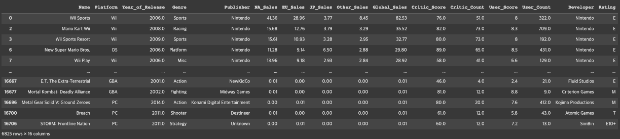

sns.histplot(x='Year_of_Release', data=df, bins=16)

sns.histplot(x='Global_Sales', data=df)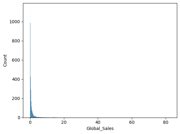

sns.rugplot(x='Global_Sales', data=df)

df[df['Global_Sales'] > 30]

gs = df['Global_Sales'].quantile(0.99)

df = df[df['Global_Sales'] < gs]

sns.histplot(x='Global_Sales', data=df)

fig = plt.figure(figsize=(20, 5))
sns.histplot(x='Global_Sales', hue='Genre', kde=True, data=df)

sns.histplot(x='Critic_Score', data=df, bins=16)

sns.histplot(x='Critic_Count', data=df, bins=16)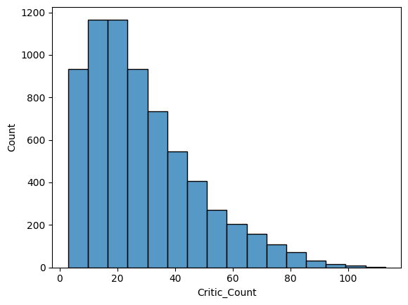

sns.histplot(data=df['User_Score'].apply(float), bins=16)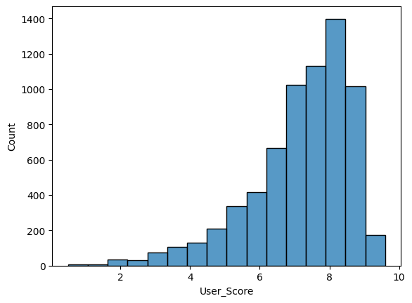

sns.histplot(x='User_Count', data=df, bins=16)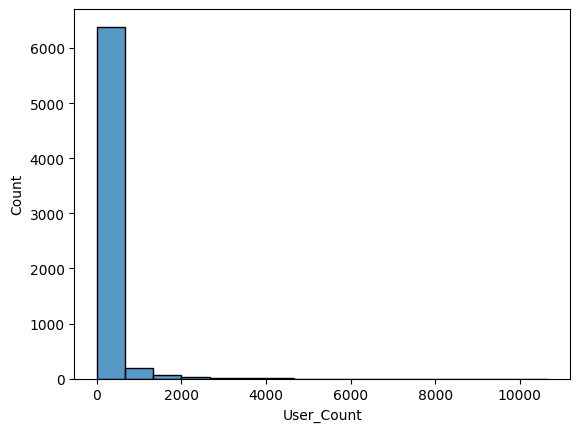

sns.rugplot(x='User_Count', data=df)

uc = df['User_Count'].quantile(0.99)

df = df[df['User_Count'] < uc]

sns.histplot(x='User_Count', data=df)

uc = df['User_Count'].quantile(0.97)
print(uc)

911.5599999999977

df = df[df['User_Count'] < uc]
sns.histplot(x='User_Count', data=df)

df['User_Score'] = df['User_Score'].apply(float)

sns.jointplot(x='Year_of_Release', y='Global_Sales', data=df, kind='hist')

sns.jointplot(x='Critic_Score', y='Global_Sales', data=df, kind='hist')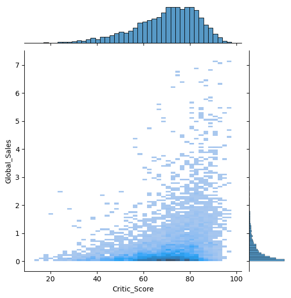

sns.jointplot(x='User_Score', y='Global_Sales', data=df, kind='hist')

sns.jointplot(x='Critic_Count', y='Global_Sales', data=df, kind='hist')

sns.jointplot(x='User_Count', y='Global_Sales', data=df, kind='hist')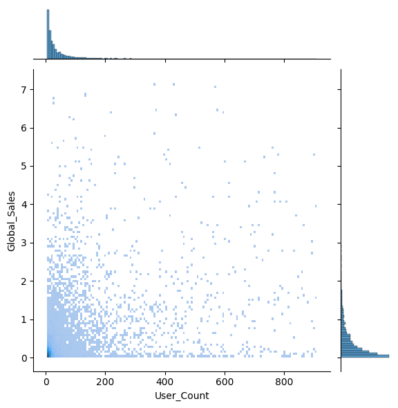

fig = plt.figure(figsize=(15, 5))
sns.boxplot(x='Platform', y='Global_Sales', data=df)

fig = plt.figure(figsize=(15, 5))
sns.boxplot(x='Genre', y='Global_Sales', data=df)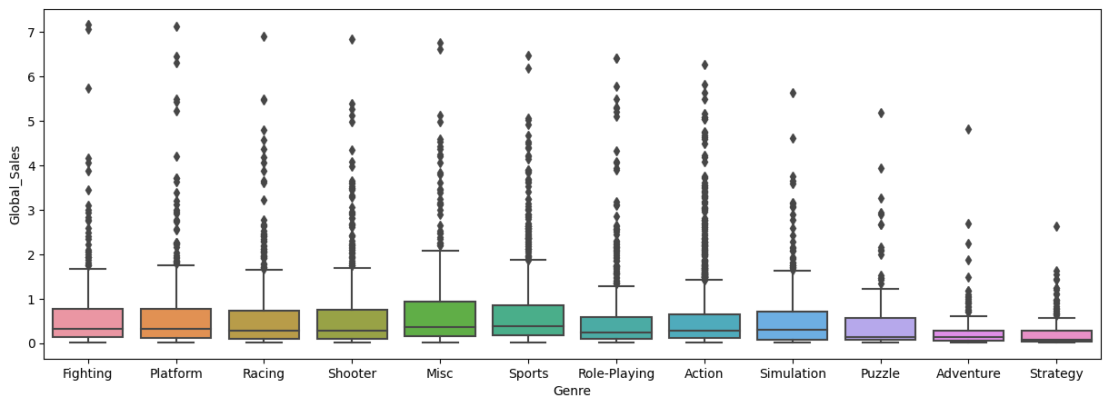

sns.boxplot(y='Critic_Score', data=df)

sns.boxplot(y='User_Score', data=df)

critic_score = df[['Critic_Score']].copy()
critic_score.rename({'Critic_Score': 'Score'}, axis=1, inplace=True)
critic_score['ScoreBy'] = 'Critics'

user_score = df[['User_Score']].copy() *10
user_score.rename({'User_Score': 'Score'}, axis=1, inplace=True)
user_score['ScoreBy'] = 'Users'

scores = pd.concat([critic_score, user_score])
scores

sns.boxplot(x='ScoreBy', y='Score', data=scores)

sns.boxplot(x='Genre', y='Critic_Score', data=df)
plt.xticks(rotation=90)
plt.show()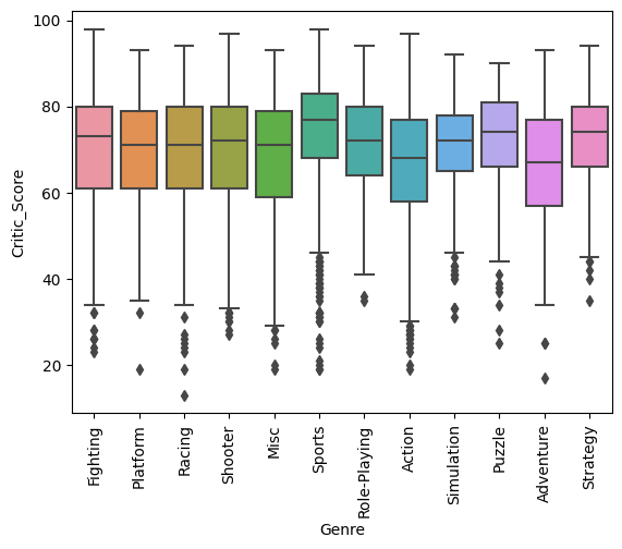

sns.boxplot(x='Genre', y='User_Score', data=df)
plt.xticks(rotation=90)
plt.show()

fig = plt.figure(figsize=(8, 8))
sns.heatmap(df.corr(), annot=True, cmap='YlOrRd')